Sonar Ray Tracing

Interactive Sonar Ray Tracing Utility

Show below is sound ray tracing utility which plots the expected path of sound waves as they propagate underwater. The path taken by sound propagating underwater is determined by reflection at the surface and ocean bottom and in between by refraction or bending which results from the variation in sound speed as a function of depth. Underwater sound speed is predominately determined by the water temperature, if this is fairly uniform then the increasing pressure as a function of depth causes a corresponding increase in the sound speed. A graph of water temperature as a function of depth is called a BATHYTHERMOGRAPH or 'bathy' for short. Water temperature profiles vary with geographic location and time of year.

This ray tracing utility allows prediction of the sound ray paths at locations all over the worlds oceans on a 15°×15° grid. The bathy typical bathy for each location has been pre-loaded, the bathys are compiled from the actual temperature data measured over a period of a month. To demonstrate the seasonal variation, the data for four different months is supplied. The bathy at any location and season may be selected and the sound propagation paths plotted for sound sources at any depth and with any initial starting angle.

The physics of underwater sound propagation is discussed in more detail in the Underwater Acoustics page. The diagrams for that article have been generated using this ray trace utility.

Using the ray tracer

Start by clicking the 'Bathy Load' tab, the bathy to be used in the ray tracing calculations may be chosen from anywhere on the globe for any of the four months, January, April, July or October. Select a month from those listed above the map, the shading color of the grid squares containing bathy data will change to indicated the month currently selected. Select a geographic location by clicking on any shaded grid square, the raw bathy data will be printed down the right hand column.

Click on the 'Bathy Plot' tab to see graphs of the water temperature and sound speed as a function of water depth. The depth scale may be adjusted to see smaller scale effects that occur near to the surface.

Clicking on the 'Ray Trace' tab shows plots the ray paths from a source which is at a user defined depth on the on the left hand axis. The source depth may be set by selecting the source depth readout and clicking and dragging the knob. Sound waves tend to travel in a diverging beam which is represented by a fan of rays, the number of rays in the fan is selectable from a single ray to a nine ray beam. The ray spacing may be set to narrow or broaden the beam spread. The graph depth scale and range scale are also adjustable.

Bathythermometric data

The water temperature profile varies with geographic location and season, it varies significantly over small changes in depth but is reasonably uniform over large distances horizontally. Although the bathy data is presented here on a 15° × 15° grid, each bathy represents the conditions only at the center of the grid square. The Haley Centre^[2] that has been used is available on a 1° grid and only the center 1° data has been downloaded for this utility. The ARGO project aims to achieve about 3° of latitude resolution. So these data can be expected to behave as if averaged over an area with a characteristic dimension of more than 3° (more than 300 km). The data has also been averaged in time, the shortest averaging time of one month has been chosen to preserve the seasonal variations. The data's vertical resolution is of the order of 1 m.

ARGO ocean monitoring project

The bathy data comes from the ARGO^[1] system of autonomous drifting buoys. There are more than 3000 of the buoys deployed around the oceans of the world, drifting 1 km below the surface, every 10 days they wake up and sample the physical ocean parameters in the water column. Their data are collected and analysed on a monthly basis and the water property profiles on a 1° grid spacing are made available at Hadley Center of the UK Met Office^[2]. The water temperature profile at the center of each square of a worldwide 15° grid has been extracted and used in the ray trace utility. Four sets of data from the months of January, April, July and October 2014 have been used in the current version to capture the seasonal variation in the sound propagation characteristics.

Application example

Locating a pinger on the bottom

Ray tracing can be used to predict the transmission pattern of an omni-directional transmitter on the sea floor, a scenario encountered when an aircraft is lost over the sea and the 'black box' acoustic pinger activates. If the bathy at Lat -23° Long 112° is selected (the search area for flight MH370, lost in April 2014) the water depth is seen to be more than 5000 m and the water temperature relatively uniform for the bottom 3 km this leads to a sound speed profile dominated by the pressure increasing with depth. If the source depth on the 'Ray Trace' page is set to the bottom, the resulting plot shows the rays encountering slower sound speeds as the propagate up from the sea floor and so they bend away from the vertical. The result is a circular shadow zone directly above the pinger with no sound from the pinger. No matter what angle the rays are launched from the source on the sea floor they can only reach the surface some 3 km away from the point directly above the pinger. A searching vessel hearing the pings will try to steer toward the strong signal but as the receiver approaches the location the signals will sharply fade inside this 3 km radius quiet zone. Ping signals will not to be heard again until the vessel is again more than 3 km away from the position above the pinger.

To see this effect Fig 1. shows a fan of rays launched from a source on the sea bed at Lat -22, Long 112 (off the West Australian coast) typical of April 2014. The rays start out at angle -90 (vertically up from the bottom), -80, -70 ... -10 (nearly horizontal). As shown in the plot the ray launched vertically is bent away from the vertical and reaches the surface 3.4 km from the spot above the source. The other angles are also bend away from the vertical forming a quiet cone 6.8 km with a diameter more than 6 km at the surface. Towing a receiver well below the surface will reduce the effective diameter of the shadow zone. With a receiver towed at 3000 m the quiet circle will be about 3 km in diameter.

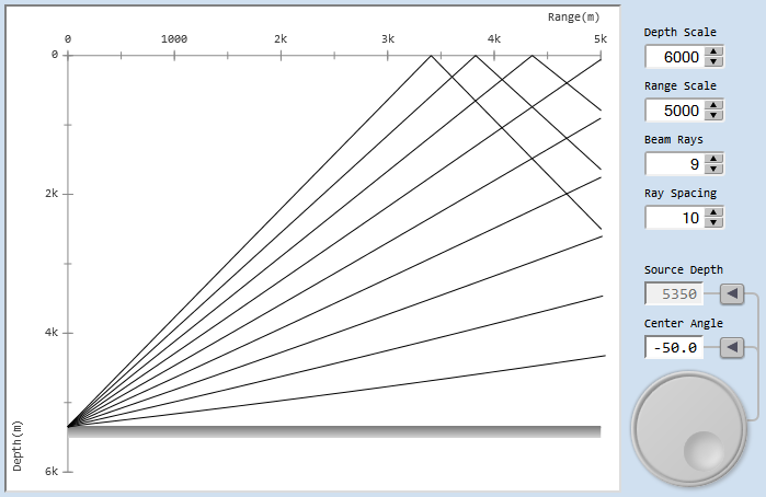
Figure 1. Sound ray pattern expected from a pinger on the sea floor showing a 3.4 km shadow zone above the source.

Acknowledgements:
1. These data were collected and made freely available by the International Argo Program and the national programs that contribute to it. (http://www.argo.ucsd.edu, http://argo.jcommops.org).
The Argo Program is part of the Global Ocean Observing System.
2. Good, S. A., M. J. Martin and N. A. Rayner, 2013.
EN4: Quality controlled ocean temperature and salinity profiles and monthly objective analyses with uncertainty estimates. Journal of Geophysical Research: Oceans, 118, 6704-6716, doi:10.1002/2013JC009067
Data Version number (EN4.0.2), downloaded 28Apr15.