Zoom FFT

Basic principle of the Zoom FFT

The zoom FFT (Fast Fourier Transform) is a signal processing technique used to analyse a portion of a spectrum at high resolution. Fig. 1a shows the spectrum of a real signal, with the region of interest shaded. The steps to apply the zoom FFT to this region are as follows:

• Frequency translate to shift the frequency range of interest down to near 0 Hz (DC), as shown in Fig. 1b.
• Low-pass filter to prevent aliasing when subsequently sampled at a lower sample rate; see Fig. 1c.
• Re-sample at a lower rate.
• Perform an FFT on the re-sampled data. Multiple blocks of data are needed to produce an FFT of the same length. The resulting spectrum will now have a much finer resolution bandwidth compared to an FFT of non-zoomed data, as shown in Fig. 1d.

Background Information: Spectrum of a real signal

If a time-domain signal is real (ie. imaginary components are 0), such as generated by a physical process, its spectrum will consist of an EVEN real part and an ODD imaginary part. EVEN real components mean that the amplitude of the real values at corresponding positive and negative frequencies are equal. ODD imaginary components mean the imaginary negative frequency components have equal amplitude but opposite sign to the positive frequency values. Fig. 2 shows the spectrum of a real signal.

Frequency translation

Moving a signal to a different frequency has long been used in amplitude-modulated (AM) radio signals, where an audio-frequency signal is mixed with (multiplied by) a high-frequency carrier. Multiplying signals in the time domain is equivalent to convolving their spectra in the frequency domain. Consequently, a copy of the audio spectrum appears centered on the carrier frequency in the RF portion of the spectrum.

Therefore, if \(ω\) is the angular frequency in the center of the region to be analyzed, multiplying by \(cos(-ωt)\) can be expected to shift the region of interest down in frequency so that it is centered at 0 frequency.

Fig. 5 shows the result of multiplying by cos(-ωt).

Unfortunately, a second, frequency-reversed copy of the spectrum is also present because the Fourier transform of cos(-ωt) has two delta functions: one at \(-ω\) and one at \(+ω\). The convolution with the \(-ω\) delta function shifts the signal spectrum down in frequency as desired, but the convolution with the \(+ω\) delta function shifts a second copy of the signal spectrum up in frequency placing negative frequencies around \(-ω\) up to 0 Hz.

This second copy of the signal spectrum must be eliminated, as it corrupts the information around 0 Hz. To accomplish this, the convolution must be performed using just a single delta function. This can be achieved by using a sum of \(cos(ωt)\) and \(sin(ωt)\). \(sin(ωt)\) has the same frequency components as \(cos(ωt)\) but has an ODD spectrum, meaning it has a negative delta function at \(ω\) and a positive delta function at \(-ω\), which lie in the imaginary domain. Multiplying \(sin(ωt)\) by \(i\) would converts all imaginary points to their negative real equivalent \((i*i = -1)\), see Fig. 6. Thus, \(cos(ωt) - i\sin(ωt)\) should produce a frequency spectrum comprising just a single real delta function at \(-ω\), see Fig. 7.

Multiplying the signal by \(cos(ωt)*-i\sin(ωt)\) is equivalent to convolving its spectrum with the single delta function at \(-ω\), producing the required shifted spectrum.

Note that:

so the formula is usually written as:

Fig. 8 shows the result of convolving the real signal with the delta function at frequency \(-ω\).

Frequency translation algorithm

If the digital time domain real signal is represented by X_k, where the subscript 'k' represents successive time domain samples, then the array X(real) contains all the signal samples. No X(imag) array is necessary as all values would be 0 for a real input signal. The frequency shifted signal, Y, will be a complex time-domain signal given by:

Yk = Xk(real) * cos(ωt)k - iXk(real) * sin(ωt)k.

Yk(real) = Xk(real) * cos(ωt)k
Yk(imag) = Xk(real) * -sin(ωt)k.

As with all complex number manipulation, the separation into real and imaginary components is purely notation; the two arrays store the real and imaginary components, and corresponding elements from each array are treated as the components of a single complex value in all calculations. The multiplication by i is implicit, by placing the data in the Y(imag) array, all subsequent calculations treat Y(imag) array elements as possessing an i coefficient.

Frequency translation source code

Using JavaScript as a demonstration language, here is the code to frequency-translate a time-domain signal:

const Np = yReal.length;      // number of data points in the data buffer
const dT = 1.0/Fsmp;          // Fsmp is the sample frequency
// Fc = center frequency of spectral region to be zoom analysed

for (let k=0; k<Np; k++)
{
  yReal[k] = xReal[k]*Math.cos(2*Math.PI*Fc*k*dT);
  yImag[k] = -xReal[k]*Math.sin(2*Math.PI*Fc*k*dT);
}

Frequency translation of complex time data

If the time domain data to be frequency-translated is already complex, meaning the imaginary components of the samples, X(imag) are not all 0, then the multiplication by e^-iωt becomes a complex multiplication:

Input:

Xk(real) + iXk(imag)

Output:

Yk = (Xk(real) + iXk(imag)) * (cos(ωt)k - isin(ωt)k)

ie.

Yk(real) = Xk(real).cos(ωt)k + Xk(imag).sin(ωt)k
Yk(imag) = Xk(imag).cos(ωt)k - Xk(real).sin(ωt)k

Low pass filter

Multi-pass filtering

The choice of filter characteristics will depend on the amount of 'zooming' required. An increase in resolution of 4 or 5 may be sufficient; on the other hand, zoom factors of 50 or more may be required. The most flexible way to address the filter stage of the Zoom FFT is to use a short FIR (finite impulse response) anti-aliasing filter, decimate (sub-sample) the output data, and then filter again - usually with the same FIR coefficients before decimating once more. Typically the frequency resolution is increased by a factor of about 4 for each pass.

Filter parameter selection

An example may be the easiest way to illustrate the technique. Assume the following values:

Input sample frequency = 65536 Hz (powers of 2 make the frequency bin spacing nice numbers)
Decimation rate  = 4              (save every 4th point; first pass decimated sample rate is 16384 Hz)
Output dynamic range = 96 dB       (gives a clean signal for a 16-bit DAC)

An anti-aliasing filter is required before decimation. The filter cutoff frequency should be chosen as high as possible without pushing the transition region so high that its alias, folding back from the Nyquist rate, reaches the filter pass-band. Aliases at higher frequencies will fall in the pass-band, but they will be attenuated by at least 96dB. Since the filter cutoff frequency lies in the middle of the pass-band edge and the stop-band edge, it should be chosen as Fs/2. With this cutoff frequency, half of the transition region will alias back from Fs/2 falling wholly within the unaliased half of the transition region.

Spectrum analysers typically maintain a display and measurement pass band comprising 400 point out of the 512 positive frequencies of a 1024-point FFT. This means that with a sampling frequency of 65536 Hz, the frequency bin spacing is 64 Hz so the 400-bin pass-band will span 6400 Hz (after decimation), and half of the transition band is 1792 Hz (8192-6400).

The width of the transition region is determined by the number of points in the FIR filter. The filter length should be as small as possible for efficiency, ie. small compared to the length of the FFTs used in the filtering process. If a 1024 point FFT is used, a filter width of around 100 points would be acceptable.

FIR filter design using the Kaiser-Bessel window method is well suited for this type of application. A description of this method and an interactive filter design utility are available on the FilterDesign page, where various cutoff frequencies and filter length can be tested and their resulting filter spectra displayed.

Selecting a 115 point filter gives a half-transition width of 1760 Hz, so a cut-off frequency of 8.19kHz the desired pass-band of 0 to 6400 Hz.

Fig. 9 shows the filter frequency response as it would appear on the FilterDesign page. Fig. 10 illustrates how the filter cutoff frequency and transition bandwidth affect the signal's frequency response after decimation.

Frequency domain filtering

The impulse response of the desired filter having been calculated, it remains to perform the filtering. This may be done by direct convolution of the time domain data with the impulse response of the FIR filter, a computationally intensive method. Alternatively, the equivalence of convolution in the time domain to multiplication in the frequency domain can be used to exploit the efficiency of the FFT algorithm.

The steps in frequency domain filtering are as follows:

• Transform the FIR filter impulse response to the frequency domain using the FFT.
• Take the next block of time domain signal data and transform it to the frequency domain using the FFT.
• Multiply the signal spectrum and the FIR filter spectrum point by point.
• Take the inverse FFT of the result, converting the signal back to the time domain, and save the filtered data to the output buffer.

The last three operations are then repeated until the input data is exhausted.

Overlap-save filtering

When directly convolving in the time domain, the first and last few points of the input data do not get filtered correctly. This can be explained as follows: if the length of the filter's impulse response, M, is 113 points, then Np = (M-1)/2 is 56 points. Convolution takes 56 points before and 56 points after each input data point, multiplying them by the corresponding points in the filter impulse response. These product values are then summed to generate a single filtered data point. Clearly, point number Np (=56) is the first point in the buffer with 56 valid preceding points; similarly, the point 56 places from the end of the buffer is the last that can be correctly filtered.

In frequency domain filtering, the FFT of a data block produces the Fourier transform of a signal corresponding to that block of time domain points repeated end-to-end. Consequently, filtering the first 56 points of the FFT buffer uses data points from the end of the buffer as part of the convolution. Similarly, the last 56 points use data from the beginning of the buffer. As a result, 113 points of each FFT buffer are corrupted and should be discarded. If the FFT is 1024 points long, only 912 (1024 - 112) points should be saved. To compensate, the next 1024 point block selected from the input should overlap the previous set by 112 points to avoid gaps in the output buffer. While the first and last 56 points of the entire input stream cannot be fully filtered, the overlap-save method correctly generates all the data that a direct time-domain convolution would produce.

A vital detail of the overlap-save method is that the subset of points from the output buffer that are uncorrupted depends on how the impulse response is positioned in the FFT buffer prior to its transformation. If an impulse response of 113 points is placed in the first 113 points of the FFT buffer, then after multiplication and inverse FFT, the uncorrupted data will reside in the block from point 113 to 1023. Note that positioning the impulse response this way introduces a phase shift in the output data relative to the input buffer. Specifically, the 113^th point in the FFT output is the filtered version of the 56^th point in the input buffer. While this may not matter for some applications, it is significant if arrival time must be measured relative to the start of the input buffer.

To avoid this phase shift, the recommended practice is to place the center point of the impulse response at the start (bin 0) of the FFT buffer, placing the first half of the impulse response (points 0 to 55) at the back of the FFT buffer (see Fig 13). . If bin indices are maintained properly between input and output copies, the uncorrupted data points after the inverse FFT will run from index 56 to 1023-56. These should be saved directly to indices 56 through 1023-56 in the output buffer, while the first 56 points of the output buffer are ignored.

Fig. 11 shows a schematic diagram of overlap-save filtering. The FIR impulse response is shown as green areas of a time domain buffer, which is then transformed via FFT. Filtering proceeds by taking the FFT of a slab of data from the long input buffer (shown in red), multiplying these frequency domain data by the FFT of the filter impulse response, and taking the inverse FFT. The uncorrupted center section (shown in blue) is then saved to the output buffer. The next slab of input data overlaps the previous section (as shown by the darker red block), and the process repeats.

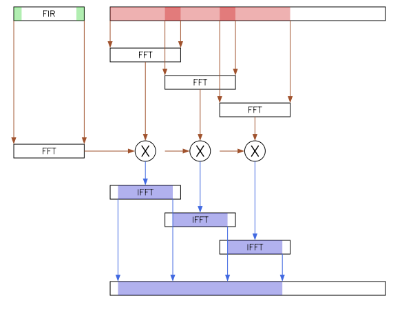
Figure 11. Schematic diagram of overlap-save filtering.

Sub-sampling

After anti-alias filtering, the time domain data is sub-sampled. Assuming a sub-sampling rate of 4, the buffer length of the signal data is now one quarter of the original length. If sufficient data remains, the filtering and sub-sampling process can be repeated to zoom in further on the region of interest (now shifted near 0 Hz).

The anti-aliasing filter coefficients required for a second sub-sampling by 4 are identical to those previously generated. With a sampling frequency of 16384 Hz (65536/4) and a low-pass cutoff frequency of 2048 Hz (8192/4), filtering the sub-sampled signal a second time with the same coefficients yields a spectrum ready for decimation down to 4096 Hz, maintaining a clean pass-band of 1600 Hz (6400/4).

Zoom FFT

If two pass filtering is performed as described, followed a 1024-points FFT, the resulting spectrum from 0 to 1600 Hz provides a zoomed view of the original region of interest. The frequency resolution of this zoomed spectrum will be 4 Hz (4096/16) sixteen times finer than the original 64 Hz (65536/1024).

To demonstrate the complete process a data buffer of 20,000 points has been created containing random noise added to two high frequency tones with frequencies around 19 kHz.

Fig. 12 shows the sample spectrum of the raw data buffer.

Fig. 13 shows the result of the Zoom FFT process. The center frequency of the spectrum is shifted to 19 kHz, two passes of the anti-alias filter and sub-sampling process applied using the filter coefficients calculated above, and a sub-sample of 4 is used, improving the frequency resolution from 128 Hz to 8 Hz.

Zoom FFT example source code

The source code to generate the Zoom FFT output whose spectrum is shown in Fig. 13 is given below.

function genTone2(buf)
{
  const fs = 65536,
        f1 = 18811,
        f2 = 18925,
        dT = 1/fs,
        PI = Math.PI;

  for (let i=0; i<buf.length; i++)
  {
    buf[i] = Math.sin(2*PI*f1*i*dT)+Math.sin(2*PI*f2*i*dT)+Math.random()+Math.random()-1;
  }
}

function zoomFFT(cvsIDa, cvsIDb)
{
  const Fc = 19000,    // zoom frequency
        tSize = 1024,  // FFT size 
        Fs = 65536,    // sample freq
        Fa = 0,        // anti-aliasing filter parameters
        Fb = 8190,
        M = 115,
        Att = 96,
        coeffs = calcFilter(Fs, Fa, Fb, M, Att),  // generate anti-aliasing filter
        Np = (M-1)/2,  // half filter length of data at front and back of buffer is corrupted 
        sigBuf = new Array(24000),
        opReal = [], opImag = [],
        aReal = [], aImag = [];
  let tBufLen = sigBuf.length;  // signal buffer length

  genTone2(sigBuf);    // generate the test signal

  // Zoom FFT starts here
  freqTranslate(sigBuf, aReal, aImag, tBufLen, Fs, Fc);
  tBufLen = overlapSaveFilter(coeffs, aReal, aImag, opReal, opImag);  // anti-alias filter
  // 1st filter, sub-sample pass
  for (let ip=Np, op=0; ip<tBufLen; ip+=4, op++)    // sub-sample by 4
  {
    aReal[op] = opReal[ip];
    aImag[op] = opImag[ip];
  }
  tBufLen = overlapSaveFilter(coeffs, aReal, aImag, opReal, opImag);  // anti-alias filter  
  // 2nd filter, sub-sample pass
  aReal.length = 0; // reset array
  aImag.length = 0;
  for (let ip=Np, op=0; ip<tBufLen; ip+=4, op++)  // sub-sample by 4
  {
    aReal[op] = opReal[ip]; 
    aImag[op] = opImag[ip];
  }
  // zoomed complex time domain data now in aReal, aImag

  // for diagnostics only, grab a buffer full of time data
  plotSpectrum(cvsIDa, sigBuf, [], tSize, Fs);
  // for diagnostics only, grab a buffer full of zoomed (complex) time data
  plotSpectrum(cvsIDb, aReal, aImag, tSize, Fs/16, Fc);
}